Images may be blended together using mathematical operations (add, subtract) coupled with Boolean operations (OR, AND) to enhance the image or extract information (Figure 10). For example, if the pasted image is subtracted from the first, a pseudo-relief image is created. If the second image is combined with the first using the Boolean OR operation the structures of the image are outlined. By pasting a copy of an image onto itself and shifting it 1 pixel a composite image can be made.
Linear Operations - Filtering
Extracting features from an image requires a different approach. The image processing program must ‘search’ the entire image pixel-by-pixel using a specific rule, such as smoothing or finding edges, and create a resultant image with the features highlighted, or at least evident. To achieve this, a small feature, or ‘kernel’, of size 3×3 up to 9×9 pixels (or more) multiplies every pixel in the image by their corresponding kernel position, sums the results, and places that result in the central pixel position. The kernel then moves to the next position in the source image and repeats the process. The pattern of values in the kernel dictates the feature revealed in the image. The process of multiplying each pixel (or voxel) an image by kernel values is called convolving the image in the spatial domain (designated as ‘*’). This is the process of filtering an image.
For example, the Laplacian 5×5 edge-detecting filter has a convolution kernel that looks like this:
1
1
1
1
1
1
1
1
1
1
1
1
24
1
1
1
1
1
1
1
1
1
1
1
1
During filtering this kernel is moved over every pixel in the image. The image pixel and its surrounding pixel values are multiplied by the corresponding values in the convolution kernel, the values added, then divided by the number of positions in the kernel. This (intensity) value then replaces the original image pixel. The kernel then shifts one pixel and the process starts anew.
A new image is created with the convolved pixel values. Using Laplacian filtering edges in the original image can be elucidated. Common filtering operations such as sharpening and smoothing use the operation of convolution.
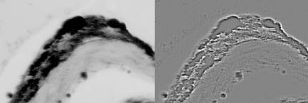
Convolution using an edge detection filter. The original image on the left was filtered with the Laplacian filter.
Filtering in the Frequency Space
As convolution kernels get larger the mathematics involved in the convolution operation becomes too cumbersome for computers. This is especially true for sharpening complex out-of-focus microscope images. In this case the convolution kernel is the image of the blur function (Point Spread Function) and is the same size and bit-depth as the images themselves. Using the convolve function (image * kernel) is too costly in CPU time to be practical. The Fourier Transformoperation solves this problem. Convolution in the spatial domain is equal to multiplication in the Fourier (frequency) domain:
g(x,y) * f(x,y) = G(u,v)F(u,v)
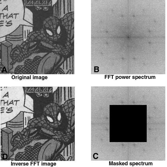
Figure 12. Fast Fourier Transform (FFT) of an image. The original image was transformed into the frequency domain resulting in the power spectrum (B). Performing an Inverse Fast Fourier Transform from the 128x128 pixel area outlined (C) results in the filtered image in D. The Black Mask in C permits an inverse FFT using only the frequence data under the mask. Outside of the mask is high-frequence image data. Note the decreased half-tone screen. Note. The MASK must be white when using FIJI.